What the Loss Landscape Tells You About Generalization

A trained neural network sits at a minimum of its loss function. What’s less obvious is that the shape of that minimum, sharp or flat, predicts whether the model will generalize.

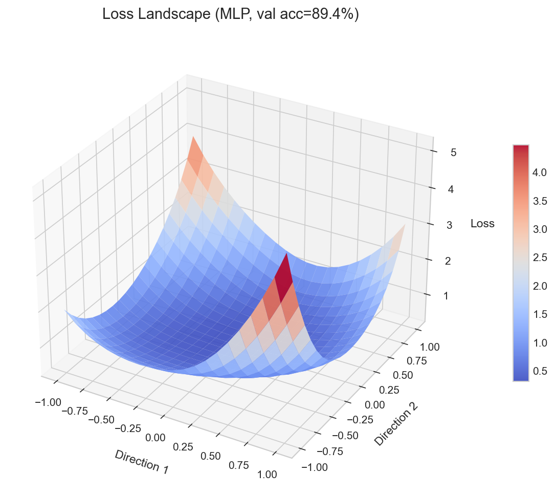
I built a tool to visualize this directly. Train an MLP on FashionMNIST with different hyperparameters, perturb the final weights along two random directions, compute the loss at each point, and plot the resulting surface. The geometry is immediate: some configurations produce tight, steep valleys. Others produce wide, gentle basins.

The loss landscape is high-dimensional. We see a slice.

The full loss landscape lives in weight space, one dimension per parameter. For even a small MLP, that’s tens of thousands of dimensions. You cannot visualize it directly.

The standard approach, from Li et al. 2018 (“Visualizing the Loss Landscape of Neural Nets”), is to pick two random direction vectors in weight space and sweep perturbations along them. This gives you a 2D slice through the landscape centered at the trained weights. It’s a projection, not the full picture.

A 2D slice through a sharp minimum looks sharp. A slice through a flat minimum looks flat. The qualitative character survives projection.

Filter normalization changes everything

If you generate random perturbation directions naively, layers with large weight norms dominate the perturbation. The landscape looks artificially sharp because one layer is being pushed hard while others barely move.

Li et al. solved this with filter normalization: scale each direction vector so its norm matches the corresponding layer’s weight norm. This ensures each layer contributes proportionally to the perturbation. Without it, you’re comparing apples to oranges across layers.

The difference in the resulting plots is striking. Raw perturbations produce jagged, spiky surfaces. Normalized perturbations produce smooth surfaces where the geometry reflects actual landscape curvature, not layer scale artifacts.

Sharp minima overfit. Flat minima generalize.

This is the core insight. A sharp minimum means small perturbations to the weights cause large jumps in loss. The model is fragile. The training data pushed it into a precise configuration that doesn’t transfer.

A flat minimum means the model is robust to perturbation. Nearby weight configurations produce similar loss. This robustness correlates with generalization because the test distribution is a perturbation of the training distribution, in a sense. A model that tolerates weight perturbation tends to tolerate distribution shift.

This connection has been studied extensively. Keskar et al. (2017) showed that large-batch training converges to sharp minima with worse generalization. Foret et al. (2021) turned the insight into an optimizer, SAM (Sharpness-Aware Minimization), which explicitly seeks parameters where the worst-case loss in a neighborhood is low.

Hyperparameters control the geometry

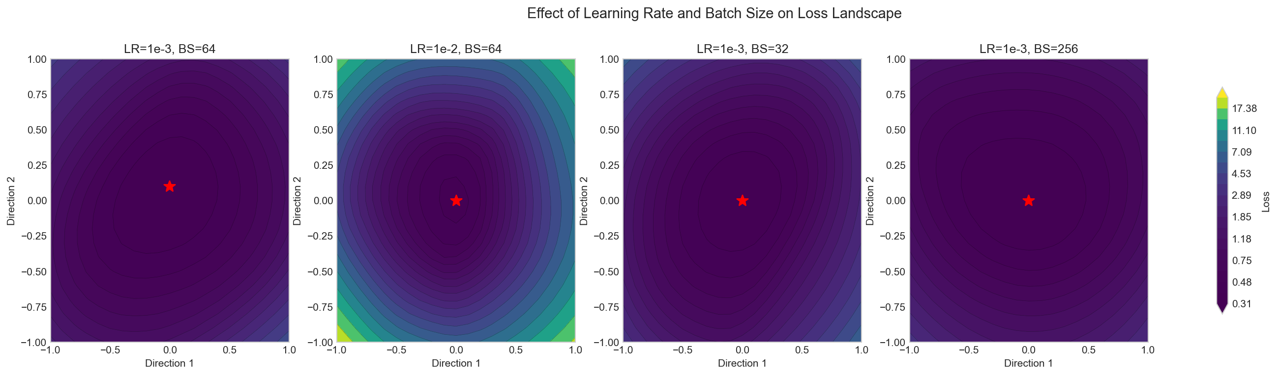
Two hyperparameters have the most visible effect on landscape shape: learning rate and batch size.

Learning rate. A large learning rate acts as implicit regularization. The parameter updates are large enough to bounce out of sharp minima, which have steep walls and narrow basins. Only flat minima are stable under large steps. This is why learning rate warmup works: start small to avoid divergence, then increase to escape sharp regions. Cosine decay then gradually reduces the rate to settle into the flattest reachable minimum.

Batch size. Small batches produce noisy gradient estimates. That noise serves the same function as a large learning rate. It destabilizes sharp minima. The model gets pushed out of narrow valleys and toward flatter regions. Large batches produce cleaner gradients that can settle into sharp minima undisturbed.

The project trains four configurations (high/low LR crossed with large/small batch) and plots their landscapes side by side. The visual difference is clear. High LR with small batches produces the widest, flattest basin. Low LR with large batches produces the sharpest.

Quantifying sharpness

Looking at surfaces is informative but subjective. The project also computes a sharpness metric: the maximum loss in a neighborhood around the minimum. Formally, for a radius epsilon around the trained weights, sharpness is max_loss_in_ball - loss_at_minimum.

This number makes comparison concrete. The sharpness bar chart across the four configurations confirms what the surface plots suggest. It also connects directly to the SAM objective, which minimizes exactly this quantity during training.

Try it

git clone https://github.com/amaljithkuttamath/loss-landscape.git
cd loss-landscape
python -m venv .venv && source .venv/bin/activate
pip install -r requirements.txt
python run.py --grid-size 31 --device cpu

This trains all four configurations and saves plots to results/. The grid size controls resolution. 31 is a good balance between detail and runtime. Bump it to 51 if you want smoother surfaces and have a few minutes to spare.

The outputs are four plots: a 3D surface, a contour map, a side-by-side comparison across hyperparameter configs, and the sharpness bar chart.